Net adjustment contents

---

Net adjustment .TNA

Topocad Net adjustment is based on calculations using the Least Squares Method, and a number of functions have been created for this to bring in data in appropriate ways and as methods for searching for errors. There are also a range of functions to customize the appearance of the results you want to present.

Entry data is based on a purge having been made to Topocad's survey data file using the SUR file format, and this data is then imported to the net adjustment; but entering data directly to the net adjustment measurements works equally well.

The known points are loaded from the preset polygon point file (default is Topocad.PP) but you can also enter known coordinates under the New Points tab.

Load survey data to net adjustment

The net adjustment uses Topocad's normal survey data protocol (*.SUR) as a basis for the observation. The survey data file of individual observations, observation series, free stations, traverses, detail observations as well as repeated observations of the same object.

To load the observation to the net adjustment form:

1. Create a new net adjustment file from File|New - Net adjustment.
2. Import data from File|Import|File and select your survey data file. Note that it must be closed
3. Select the instrument you have used.
4. Select the stations and the type of data for import. See below.
5. The imported measurements appear under the Observations tab,
6. where you can also enter or edit other measurements.

Instruments

Enter the instrument to be used in the survey data file. You must have defined the instrument under File|Project Settings|Instruments. Click the Add button to enter an instrument name and then define the properties the instrument has. Note that the instrument must have been defined before importing the survey data file.

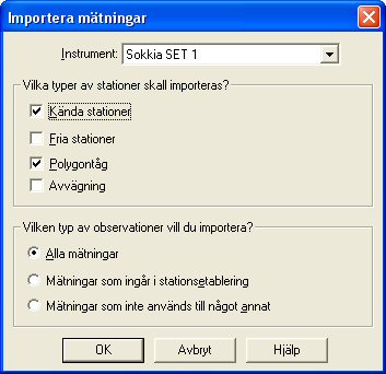
Settings for import - What kind of Stations would you like to import?

• Known stations (polar configuration)
• Free Stations
• Traverse (standard mode, only the points that are highlighted with the traverse survey type are usually calculated)
• Leveling

Settings - What kind of observations?

• All observations - also includes detail points.
• Observations that are part of the station establishment, i.e. those that have the survey type "station" and have been coded with the point type backsight or polygon point.
• Observations that are used for something else. This means those points that have been marked with the survey type "Other".

Settings

You can make several speed settings under Net adj.|Settings in the main menu. These settings do not affect the survey data/measurements but only give the program instructions on how to calculate. This means that even though plane and height are to be calculated for a measurement, the speed setting is to be set to plane alone.

You can make these settings under three different tabs:

General

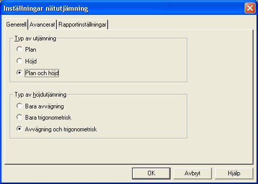
Type of adjustment:

• Plane
• Height
• Plane and height

Type of height adjustment: (only when adjusting height or plane and height)

• Only leveling (only levelled survey data is included in the height adjustment)
• Only trigonometric (only trigonometric observations included)
• Leveling and trigonometric (both survey types included)

Advanced

Speed settings

These speed settings control the calculation and take precedent over the settings made for each individual observation under the observation tab. The advantage of this is that you are sure that the selected type of calculation really applies to all observations. In order to use the individual settings for each individual observation, you must select Own settings in this list.  

Use project settings
Use the settings made under Cordinate System. It is principally the Coordinate tab that is of interest when selecting the coordinate system. If this is not Local, an ellipsoid correction will occur (height correction projection of length of the ellipsoid) and the projection correction for all observations.

Own settings
Use the settings under the Observations tab exclusively, i.e. if the ellipsoid or projection correction is to be calculated for each observation.

Free adjustment
Release all points to ensure the error for the known coordinates does not affect the net. This is good for a local net that is to be as tension free as possible, or if you suspect that there is an error in the known coordinates. If this adjustment gives good results in a well-balanced net, this indicates that all observations are OK, and that an error in a normal (forced) adjustment depends on an error in the known coordinates. Remember that an observation in a traverse of observations that ends at a known point is calculated as a detail observation in free adjustment, which means that gross errors cannot be traced for observations of this type. In order for a free adjustment to be implemented successfully, the net should be designed as loops or triangles. Traverses without loops may produce uncertain results.

Projection and ellipsoid correction is deactivated for this adjustment. If you want to carry out a free adjustment with the corrections activated, you must use the speed setting Own settings instead; select Free adjustment under Detailed settings and then select Yes for all the corrections for the observations in the observation tab.

Free adjustment, local system
You restrict the known points here to two and allow the program to calculate a bearing from the station point, which retains its coordinates. This method also removes tension in the known points, but retains the station point coordinates (all known coordinates are affected in a totally free adjustment).

Local coordinate system
Does not use corrections for projection and ellipsoid.

Unknown coordinate system
Uses a free scale to eliminate the affect of a scale error on the lengths. This method is ideal if you have major errors in the lengths and suspect that you have an incorrect Y-offset for the coordinates (affects the projection correction) or has a length gauge with a scale error. If an adjustment with free scale drastically reduces the length errors, you may assume that you have an error of this type.

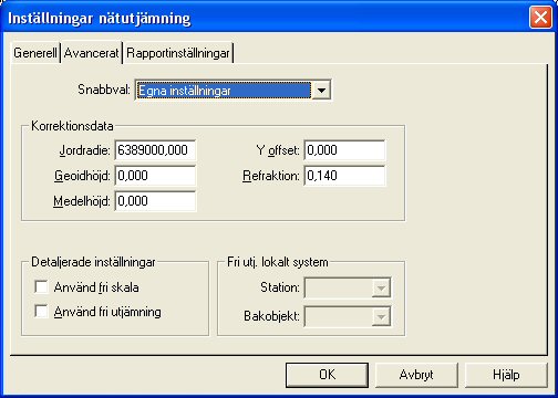
Correction data

The values specified here are inactive (grey) if you have selected a speed setting option where the values have either been loaded from the project settings (File|Settings|Project Settings) or are not used in the calculation.

Earth radius-
required for correction calculations. As a standard value 6370000 is used for Sweden. If you use a RT90 coordinate system in the project settings and have specified the Use project settings speed setting, the program will calculate an earth radius as per the formulas in HMK Geodesi Stommätning (HMK Geodetics Control Point Surveying) Chap B.1.1 and data for Bessel's ellipsoid.

Geoid height-
the height (water surface) of the geoid compared to the map projection's reference ellipsoid (Bessel's ellipsoid applies to RT90). If you use a RT90 coordinate system in the project settings and have specified the Use project settings speed setting, the program will calculate a geoid height using the geoid height model RN92.

Y offset-
offset in Y which is often 1,500,000 for RT90 coordinates to avoid negative Y values. It is very important to check this value if you allow the net adjustment to calculate the projection correction. If you use coordinates with the specified offset, but forget to specify it as Y offset, a length of 100 m will have an error of around 2.7m. In File|Settings|Project settings|Coordinate you select a system with a specified offset. This is often abbreviated; e.g. RT90 5 GON V 60: -1 means that you subtract 6,000,000 from the X-coordinate and add 100,000 to the Y-coordinate. The projection correction formulas used are described in HMK Geodesi Stommätning Chap. C2.

Refraction-
the refraction of the light in the atmosphere. The standard value for the refraction coefficient is 0.140 for Swedish conditions. The refraction influences the calculation of the height difference and is used in calculations according to the definitions in HMK Geodesi Stommätning Chap. C3.

Mean height-
if you are to calculate the ellipsoid correction but do not have the z coordinates for your points (required in the calculation), you can specify the mean height above sea level for the net you want to calculate. For a length of 1,000m, a height error of 10m will result in a correction error of just 2mm, so you only need an approximate height for the points; meter accuracy is often enough. The height correction formulas are described in HMK Geodesi Stommätning Chap. C1.

Detailed settings: (active for the speed setting Open Settings)

Use free scale-
used if you want to calculate the scale if it is unknown, for searching of scale errors in nets with major improvements for lengths, or for tests of a net with known scale to see if the specified scale factor seems to tally.

Use free adjustment-
Use free adjustment- adjusts the net without taking fixed known coordinates into consideration. Good for nets that need to be free from tension. See Free adjustment under Netadj.|Settings Speed settings. As free adjustment here occurs under the Own settings speed setting, the ellipsoid and projection correction will be carried out for a certain observation if you have specified the observation's row in the survey data tab.

Use centring error for new points

If you have used forced centring consistently during the observations (had the tripod in the same place but changed the places of instruments and prisms) you will be aiming at the exact same point that you measured from. In practice, this means that the effects of the centring error will not influence the precision of the observations. The centring error is added to the mean error of the calculated new points instead. However, when you connect to a known point, the centring point will have an effect as the known coordinates apply to the point on the ground and not the position of the tripod over the point. The program will therefore include the centring error from known points in normal mode, but not new points when calculating the observation's apriori mean error. This is closest to reality if forced centrings dominate in the net. However, if you take the tripod down for the majority of the observations, you should also take the centring errors of the new points into consideration when calculating the apriori mean errors.

To sum up this means the following: If you have used forced centring predominantly in the net, the Use centring errors for new points box should NOT be checked; whereas is should be checked in reverse position.

Explanations for Observations

An explanation of the columns follows under the Observations tab:

From Point
Select from which point you have made the observation, i.e. the station point. This may be both a known point and a free station, or a new point in the centre of the traverse.

To point
Marks the point to which the measurement is made.  This could be both a known or a new point.

Series no.
Normally you measure one direction series at a time per station and then change the station point. If you have measured in this way, you do not need to worry about this column which will then have a default value of 1 for all observations. However, if a special case occurs where you measure one more direction series from the same station straight after the first series, the series need to be separated from each other in some way. If this does not happen, the program treats both series as one which may lead to errors. We differentiate between the series by manually assigning the value of 2 in the series column to the other direction series. If we have a third series from the same station immediately after the second we assign these observations the value of 3 etc... If several station establishments occur in a row from the same point in a survey data file, the net adjustment when importing will set different series numbers automatically to separate the measurement series.

Hor. angle
Horizontal angle.

Vert. angle
Vertical angle.

Length
Slope distance. If the vertical angle field on the same row is blank, the length is treated as horizontal.

Height diff.
Measure the height difference between the from and to point. Used primarily for leveling data.

Bearing
Here you can enter a known bearing between two points. It could either be a fictitious bearing to give the net the desired orientation (turned facing north), or a bearing measured using gyrotheodolite.

Instr. elevation
Height of instrument above the point.

Refl. height
Reflector (prism) height above the point.

Instruments
Specify the instrument used, which in turn defines the precision of the observations (measured as accuracy), which is displayed under the instrument tab.

Proj. corr
Projection correction - specifies if this is to be used or not for the observation. Speed settings are available in Settings (see this chapter for a more detailed description) if you have selected Use project settings, which generally activates/deactivates this function for all observations regardless of what has been specified for each individual observation. The projection correction formulas used are described in HMK Geodesi Stommätning Chap. C2.

Ellips. corr
Ellipsoid correction - specifies if this is to be used or not for the observation. The correction reduces measured lengths to the ellipsoid. The height correction formulas used are described in HMK Geodesi Stommätning Chap. C1. Just as for the projection correction, the speed settings will take precedent over the individual settings for an observation.

Atm. corr.
Atmosphere correction to lengths. This function is affected in the same way as the projection correction to the speed settings in Settings. The corrections are calculated as follows (obtained from instrument manuals from the manufacturer in question):

Leica
ppm=281.5-((0.29035* pressure)/(1+0.00366* temp))

Trimble/Geodimeter
ppm=275-((79.53*pressure)/(273+temp))

Topcon
ppm=279.6-((79.53*pressure)/(273.2+temp))

Sokkia Laser
ppm=282.59-((0.2942*pressure)/(1+0.003661*temp))

Sokkia Reflector
ppm=278.96-((0.2904*pressure)/(1+0.003661*temp))

Pressure and temperature are specified as mbar and degrees. The lengths are then corrected by multiplying by the ppm figure. If the length is specified in km, the correction is given in mm.

Pressure
Atmospheric pressure. Consideration is taken to this only if Yes had been entered in the Atm. corr. column. If you have the values in mmhg you recalculate them to mbar by multiplying by 1.3333, which is simply done using the Search/Modify function that you activate by right-clicking.

Temp
Temperature in degrees. Consideration is taken to this only if Yes has been entered in the Atm. corr.

Weight f. length
Weight factor length. Weights for lengths are automatically calculated through the formula P= 1 / mf2, where mf is the observation's mean error that is obtained from the instrument data. This value does not need to be changed by the user. If you end up in a situation where you know that an observation is worse than expected due to external circumstances (e.g. weather, light conditions, instrument errors), or if you, for whatever reason, would like certain observations to have less of an effect on the results, you can reduce the weighting of the observation. For lengths, this is done by changing the weight factor from 1 (=unaffected) to a lower value. If we change to 0.5, for example, this particular length will affect the result half as much as normal (the previously calculated weight is halved).

Weight f. angle
Weight factor angle. See above for explanation.

Weight f. height
Weight factor height. See above for explanation. Apart from levelled heights, this can also be used for an observation of the vertical angle and length if trigonometric heights are to be used. Weights for heights are calculated for leveling automatically using the formula P= k / L where L is the length between the points in km. k is a constant that is set to one if only one instrument is used. If several instruments have been used, k is set for the observations with the best instrument to one and for the others to one divided by how many times worse the observation's instrument is compared to the best instrument (calculated from the instruments' apriori mean errors).

Use observation
This tab has a number of selections and all of them specify the observations for the current row to be included in the calculations:

 

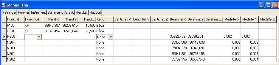
Points

Under the points tab we can see all points (known and new) that are included in the adjustment. Known points are loaded automatically from the current polygon point file when we import a survey data file or enter survey data directly in the net adjustment. Both station (from) and object (to) points are checked.

It is also possible to change the coordinates of a known point manually, and to change points from known to new points if you want these to be calculated in the adjustment and not be used as fixed points (e.g. if you suspect that the known coordinates are wrong). A new point can be made known by entering the coordinates in the columns Known X, Y, or Z. To change this, go to the Known column, where you can also enter a point as known in plane but not in height or vice versa. If the coordinates for a point have been calculated, you can lock them by changing in the known column as mentioned previously. The calculated coordinates are then copied to the columns for known coordinates.

In addition to the coordinates, there are columns for centring errors X, Y, and Z. Here you can enter a centring error that you know applies to the point irrespective of the instrument. If we have blank cells here, the values we have entered for centring errors under Instruments will apply. For a normal tripod set up, 3mm is a normal error, but if we use wall prisms for example it is lower. A free station point always has the centring error 0, but its coordinates are usually of no interest.

We can also use the centring error if we use calculated points as known points from an old adjustment. Normally, all known points have a great accuracy, but by using the point mean errors from the old adjustment, we can provide observations in relation to worse known points with a little greater margin. As a result, uncertainty from these points (with greater mean errors from the old adjustment) will have less of an impact on our new adjustment.

Following the completion of the calculation we see Calculated X, Y, and Z, as well as Mean errors X, Y, and Z for the points, that tell us the calculated position of the new points and the precision they have. For a more detailed explanation for these headings, see Report.
 

Instruments

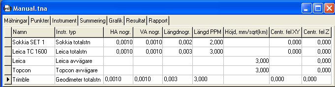
A list appears under instruments showing those instruments that have been selected when importing one or more survey data files. The type of Instrument can then be selected for each observation under the observations tab in the Instrument column.

Data on the instruments can be obtained from the relevant supplier. The weights are calculated from these values, which means that an observation with a good instrument will affect the result more than the observations with an inferior result. The values you enter are the instrument's factory tested apriori mean error (see Report).

In general you could say that it is the standard mean error in particular that is directly influenced by the instrument data, as it is a comparison with the capacity of the instrument (1.000 means that you have measured exactly at a level the instrument can handle). As a result of this, the standard and observation mean errors as well as the sigma levels vary depending on the instrument data we choose. It should also be noted that the instrument data affects how the various observations are weighted in relation to each other, i.e. how much they affect the results. NOTE: It is therefore of the utmost importance that we have specified the correct values for the instrument's data if we want reliable assessments of the quality of the net. Note that you may not specify a value to 0.0000 as this is an unreasonable value that would apply to a completely error free instrument, which makes the weights impossible to calculate.

Settings

Instr.type
Different makes of instrument handle the corrections for pressure and temperature in different ways, which is taken into consideration under this setting. See  also Atm. corr in the observations chapter.

HA Accuracy
Horizontal angle accuracy. Entered in GON (adjustable to mgon or degrees)

VA Accuracy
Vertical angle accuracy. Entered in GON (adjustable to mgon or degrees)

Length accuracy (constant)
Specified in meters (adjustable to millimeters)

Length accuracy (PPM)
Entered in PPM

centring error in plane
A centring error can either be specified for each point or generally for from and to points where the instrument is used. The centring error will give all observations that have been made using the instrument and offset in the accuracies specified above. E.g. the length accuracy will be calculated as a bit worse depending on the effect the centring errors have. If a field is blank in the centring error columns X and Y under the Points tab, the centring error specified for the instrument will be used.

centring error in height
See above.

Note that you may not specify a value to 0.00000 as this is an unreasonable value that would apply to a completely error free instrument, which makes the weights impossible to calculate.

Calculating of net

To calculate a net, go to Net adjustment|Calculation, or click on one of the Graphics, Results or Report tabs. If a change has been made to the input data or if we make our initial calculation, we see the message The net adjustment has been changed, do you want to calculate the net? under these tabs, to which you answer yes.

Note that the speed settings you have made in Netadj.|Settings apply. If you want to use your own settings for atmosphere, ellipsoid  and/or projection correction, the speed setting must be specified as Own settings.

Calculation is made immediately and you can go to the Summary, Graphics, Results or Report tabs to see the results.

View screen settings

An appropriate size to symbols for the screen depends entirely on how extensive the net is and what zoom setting you are in, which is why you have the option of adjusting the symbol size. The symbols are triangular for known points in plane, circular for new points and triangular with a circle for known points in both plane and height. Measurements are marked with straight dashes for measured lengths and angles for measured angles.

Error ellipses are obviously shown by ellipses and height errors by a vertical dash through the point. If the ellipses had the same scale as the net they would not be visible. Instead you can set the scale factor here that they are to be enlarged by in relation to the net. You can also change the colours of the ellipses and symbols.

It should also be noted that the same graphical functions are available under View as for other applications in Topocad, e.g. zoom, pan, drag, redraw etc...

Point ID with possibilities to change the size of the text. The point symbols can also be changed by going to File|Settings|System settings and selecting the Point info tab. The PointID box you can change placement, font and size of the point symbols.

Tests

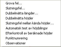
This menu has a number of tests to see if our survey data contains gross errors. The specified tests observe the descriptions in HMK Geodesi Stommätning.

Search for gross errors

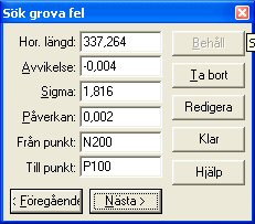Searching for gross errors enables you to run a quick check over the measurements in the net. By activating the Tests|Gross errors command, the program zooms in automatically on the biggest error in the net, that is the measurement (length or angle) that has the largest standard improvement. This is calculated in line with HMK's definition as the    so called sigma level, which is the observation's improvement divided by the observation's apriori mean error. For each measurement you can determine whether you are to edit the measurement, retain it, or erase (delete) it. Click Next to view the second largest error, and so on. If you want to return (to larger errors), click Previous.

If you specify Edit, the program skips to the measurement tab and selects the current measurement. It is then possible to edit and go back to the graphics, whereupon the question is asked if the net is to be recalculated.

Connection error

This check is manual and can be used for gross error searching by going traverse in the net. Start by clicking somewhere in the screen to form a square. By selecting point by point and then returning to the starting point, the connection error is calculated for the loop. This process gives a safe and quick check of the net, and you can quickly find any errors by using several different loops.

Undo delete of the last added point, restart by clearing memorized points.

Double measured distances

This test method searches for all distances that are measured in both directions and compares them with each other. The difference is then checked against a threshold specified in System settings. The program will immediately create a finished report with the tested distances.

Double measured heights

This test method searches for all height differences that are measured in both directions and compares them with each other. The difference is then checked against a threshold specified in System settings. The program will immediately create a finished report with the tested height differences.

Connection error between known heights

This test method automatically calculates the height traverse between known heights the program can find in the net. The total height difference for the observations are compared with the height difference between the known heights. A report is created where a comparison to the threshold is made.

Automatic test of height loops

The program automatically calculates height loops that can be created in the net. The connection errors are compared to the thresholds and are printed in a report.

Post checking of calculated heights

This test method compares the adjusted heights with the observations that were included in the adjustment. A comparison is made with the thresholds and the results are printed in a report.

Point numbering

The test method checks to see if any points have similar coordinates, which may be a sign that they are actually different names for the same point. Similar point coordinates are compared to a threshold in a report.

Measurements

The test checks if any stations have fewer than four objects (not preferable in Banverket's (Swedish Rail Adm) lattice polygon), and lengths that are only measured in one direction. These stations are listed in a report.

Known points

If we have carried out a forced adjustment (adjustment with known points locked) and had several observations designated as incorrect, this does not always need to be due to the error in the observations. It could instead be that the known points have incorrect positions. This could be due to them moving, that you have use the wrong error point, or that we have specified the wrong coordinates. All known points are calculated in the adjustment as perfect and any errors they may have are interpreted as observation errors instead.

In order to test the observations without any influence from coordinate errors, you should therefore carry out a free adjustment (all points treated as new) in order to remove all errors in the observations. This assumes that the net is linked in loops as far as possible traverses to connection points produce uncertain results for free adjustment.

If you have removed all the observation faults in the net, it simply remains to test the positions of the known points. You do this via the following steps:

• If you have selected Plane or Plane and height under Netadj.|Settings|General the known coordinates in plane are tested. If the selection is Height, the Z coordinates are tested instead.
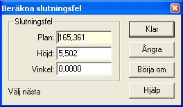
• The test starts by selecting Tests|Known points. The following window appears:

1. Here we select the points we want to test in the list first Lock/release known points. The points that are pre-checked will be included in the test. If we click the Extents button, all points will be included. The None button releases all points allowing you to make your own selection. This gives us the option of testing known points in a certain part of the net, which can be useful in expansive nets.
2. The program can then be set to stop when a calculation has been made (Only release point with greatest error) or release the worst point and recalculate until all points meet the threshold (Release points until the net is approved). The latter is as quick and easy as an initial test, but the final check should preferably be carried out point by point where you make a thorough analysis before proceeding.
3. When the program calculates length observations, you can specify under Corrections if the lengths are to be corrected for Ellipsoid and Projection. If you select Use project settings, the corrections apply that have been set generally for the project. Settings can be checked under File|Settings|Project settings|Coordinate. If you select According to settings, the settings are used for each individual observation's corrections (the Projection and Ellipsoid columns) in the observations tab. Note that these selections apply regardless of what you have set as speed settings under Net adj.|Settings|Advanced.

In order to describe other settings, we go through what happens if you start the test by pressing Calculate:

• A free adjustment is carried out. For the points to be tested, the coordinates are picked that the points were given in the free adjustment. These are incorrect in that they originate from a free adjustment, but if this is correct the points will be right in relation to each other.
• The program then takes test points coordinates from the free adjustment and transforms them so they fit as well as possible with the known coordinates for the same points.
• This is done to test in plane by moving in X and Y, rotating and, if you have selected it in the program, scale changing. Do this by selecting Congruent or Helmert as Transformation. The latter type also adjusts the scale of the free net, which means that you remove the influence of the scale error at the length gauge. If you are sure that the scale of the lengths is correct, you should use Congruent, which retains the scale of the lengths. Otherwise there is a small risk of fitting errors at the points being partially interpreted as scale errors in the calculation instead.
• For heights, the transformation takes place via the program calculating the average values for both the known and the adjusted points. The mean value is then removed from known and adjusted coordinates making both averages zero (center of mass reduction).
• For heights, mean errors are also calculated for connection height fixes even though they are not part of the free adjustment. The program then looks up the nearest adjusted height and uses the mean error's law of error propagation for the connection observations and the nearest adjusted point to set a mean error for the height fix you have connected to. Naturally, this value does not have the same certainty as the height mean error that is included in the free adjustment. However, excluding them would mean that you would not get any connection height fixes at all in the test, which is often a major disadvantage as this measurement situation occurs quite often.
• In plane position only the known points that are included in the free adjustment, i.e. connection points are excluded from the test unless the observations are over-determined in relation to them. This is due to them being uncertain in relation to the other net, where at least two unchecked observations (angle and length) are used. However, it is normal in plane mode that the connection observations are over-determined to ensure the points are included in the free net. We also have situations when just one angle is measured in relation to a known point that is a backsight. In that case this point is impossible to test and is excluded from the test.
• If the known coordinates are correct (and also the observations in the free adjustment) the adjusted and known coordinates fit exactly with each other for a transformation. If any point is incorrect, this is noticeable by it having a fitting error between the free and known coordinates. The fitting error is reported as an error divided into X and Y as well as radial (total) errors. The problem now is where to draw the boundary line for when a point is incorrect and, in connection with this, take into consideration the error sources included in the calculation. These are primarily the mean errors of the points from the transformation and the free adjustment. A point that is at the edge of the net will be more uncertain in the transformation than one in the middle.
• In order to have a tool that is as certain as possible when identifying errors, a test quota is calculated. This specifies how large the fitting error is compared to the total mean errors of the point from the transformation and the free adjustment in the direction of the fitting error. This test value can be compared with standardized improvements (sigma levels) for observations. Following this, HMK's three level principle can be applied in order to assess if a point is wrong or not. You can set the program if the limit for errors is set at factor 2 (95% error probability), 3 (99.8%) or your own level.
• When the calculation is complete, the number of points is reported that are locked or released following the calculation. In the Current point box you can see the worse point's ID and test quota together with the error in X and Y, radial (total) and the direction (bearing) in which the point has moved.
• If you click Edit, the program jumps to the point tab and positions itself on the row of the current point. This is to enable you to quickly check and, if necessary, correct any wrong coordinates for the current point. If you click Next, the second worse point is displayed and so on. Previous then goes in the other direction.
• We can also tick the box if the point is to be known (Locked) or released in the next calculation.
• You get a summary of a calculation by clicking Report. You then select the report template you want to use (normally Standard) and then get a summary of the calculation. The report shows the following details first:

• The standard mean error is then displayed, HMK's approval limit, over-determinations and K-Value for the free adjustment that form the basis of the test. Following this the same parameters are shown for the forced adjustment with all points locked and finally a forced adjustment with only the remaining locked points as known. The idea here is that you can see if the deleted points improve the net as a whole at the last adjustment.
• The data is then displayed for the point(s) that have been released. The following data is displayed:

• The next part of the report is a record of each individual search and its results. If we have set the program to only make one calculation, it is shown here. If we have selected Release points until the net is approved all the separate calculations are reported. The following data is included:

• When you have finished analyzing the results, you can print or save the results file in various formats using the icons top left. To return to the test settings, close the results window and select OK, whereupon you return to the test's initial window. If points have been released during or after the latest calculation, they are now released in the list Lock/release known points. We can now choose to change the settings, release or lock points, and recalculate.
• When we have finished with the test, we press Apply. We are then asked if we want the points that have been released in the test to be released under the point tab as well. To give known points new coordinates could be delicate and you should be aware of the consequences. The danger is that you could easily have different coordinates for a certain point in different projects, so the points that are released should not be uncertain.

Summary

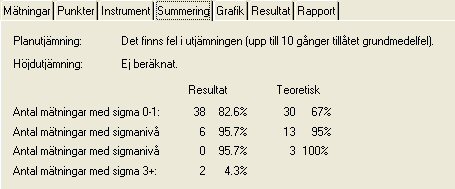
When you have made a calculation you can see the general results by selecting the Summary tab. The calculation primarily specifies if a standard mean error is approved in plane and/or height (see Report). If this is not the case, either the error is specified as large but the calculation was still possible or it was too large to allow an adjustment.

We will then identify the most important results which means that you can assess if the adjustment is to be approved or not for plane and height. Here the net's standard mean error is included, K-value, and the largest point mean error in plane (error ellipse large axis) and height. You also get the observations' largest sigma level, improvement (for angle, length, and height difference) and lowest relative redundancy (individual K-value). See the description of these parameters in the Report chapter.

In addition to this, a summary of the observations' sigma levels is listed to ensure that you can assess whether the observations contain gross errors. The distribution of the sigma levels is compared with the theoretical values that an average calculation would give.

Results

You can view the most important values under results which specify how the latest adjustment went. In addition to received and permitted (as per HMK) standard mean errors, we see how many gross errors we are estimated to have in the net, and a comment that describes how the adjustment went overall. If it was not possible to implement, the reason for this is given.

Report

The report is divided into a number of main headings. If these headings are included, and the type of data they cover, depends on the report settings you select. The data the program can include in the report are as follows:

Total

Statistics

Number&
Here you specify the number of horizontal angles, vertical angles, direction series, horizontal lengths, measured distances and known points in plane and height. Also shown are max, min and mean values for the following values: sigma levels, length improvements, horizontal angle and bearing improvements, height improvements, largest influence in plane and height  and point mean error in plane and height.

Known points

PointID
Name of point.

X, Y, Z coordinate
Specified known coordinates for the point.

Centr. incorrect X, Y, Z
Specified centring error for the point.

New points

Observations

 
Save polygon points

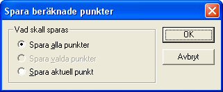
By placing yourself under the New points tab and then going to the Netadj.|Save points to PP command, the calculated points in the current polygon point file (.PP) are saved. Note that you must have selected the Points tab in order to use this function.

You can select between saving all new points, the current point you have selected or a range of points. If you want to save points in a new file, you create a new polygon point file via New|Polygon points and then connect it to the project via Settings|System settings|Observation whereupon you select the new file. Finish by saving the points as per the description above.

Lock all calculated heights

When the height adjustment has been carried out, you can then lock all calculated heights by selecting Netadj.|Lock all calculated heights. This locks all available heights, and can be used to trace all incorrect instrument heights and signal heights.

Save net adjustment to drawing

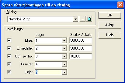
Going to the Net adjustment|Save net adjustment to drawing command saves all detail points and also over-determined points down to an optional drawing. Here you specify the drawing by specifying a previous save, an open or a completely new drawing.

Note that the codes of the points can be used to sort at different levels which is an excellent option for separating data from each other.